StableQAT, a Fourier surrogate for the rounding gradient
Quantization-aware training fakes the gradient of the rounding step; almost everyone fakes it with the straight-through estimator (pretend round's derivative is 1). StableQAT replaces that constant with a smooth surrogate derived by rotating the rounding staircase into a triangle wave and Fourier-expanding it, with STE as the zero-amplitude special case. I read the Microsoft repo and verified the surrogate's math: the STE limit, the amplitude conditioning boundary, and the bounded-variance theorem.
- Authors
- Tianyi Chen, Sihan Chen, Xiaoyi Qu, Dan Zhao, Ruomei Yan, Jongwoo Ko, Luming Liang, Pashmina Cameron · arXiv preprint (ICML 2026 format) · 2026
- Audit
-
reference code read at
4760535· July 18, 2026 - Claims
- Note
Core insights. Quantization-aware training runs the forward pass through a hard rounding step, whose derivative is zero almost everywhere, so training needs a fake gradient for it. The universal choice is the straight-through estimator (STE): pretend rounding was the identity, so its derivative is 1. StableQAT changes exactly this one thing. It rotates the rounding staircase 45 degrees into a triangle wave, Fourier-expands that, and rotates back, producing a smooth per-element surrogate gradient that is largest at the rounding boundaries and smallest at the cell centres. STE falls out as the zero-amplitude member of the family. The forward pass is untouched (plain LSQ round-and-clamp), so this is a training-time-only change with no inference cost and, because the surrogate is a cosine rather than the exp inside soft quantizers like DSQ, almost no training overhead. On Llama-3.2-1B and 3B at 2 to 4 bits it beats ParetoQ (STE) and DSQ (soft rounding), by the most at 3 bits, and with tighter variance across learning rates. I verified the surrogate’s mathematics; I did not re-run the training.
Method
The one gradient QAT has to invent
The mechanics of QAT are in the ParetoQ note: keep full-precision shadow weights, quantize them on every forward pass so the loss sees the low-bit weights the deployed model will use, and update the shadow copies. The snag is the rounding operator. is a staircase: flat between half-integers, with a jump at each. Its derivative is 0 on the flats and undefined (an impulse) at the jumps, so a real gradient would be zero almost everywhere and nothing would train. STE papers over this by pretending, in the backward pass only, that . It works well enough that essentially every QAT method uses it, but it is a lie about the shape of the operator, and at 2 to 3 bits, where each weight has only a few destinations and the loss surface is jagged, the lie starts to cost stability.
StableQAT’s claim is that you can do better than the constant 1 without paying for a soft forward pass. Its surrogate is what it calls a Rotated Damped Fourier Surrogate (RDFS); the code, less grandly, calls it “sine soft quantization.”
Rotating the staircase into something Fourier can eat
The derivation is the part I found genuinely nice. Plot the rounding map as points with : a staircase. Rotate the coordinate frame 45 degrees counterclockwise, setting and . The staircase straightens into a periodic triangle wave with period (the paper says, and the left panels below show it). A triangle wave is periodic and square-integrable, so it has an ordinary Fourier series, and its derivative back in the original coordinates has a clean closed form. Carrying the first Fourier term through the inverse rotation and the chain rule gives the first-order surrogate the code actually uses for :
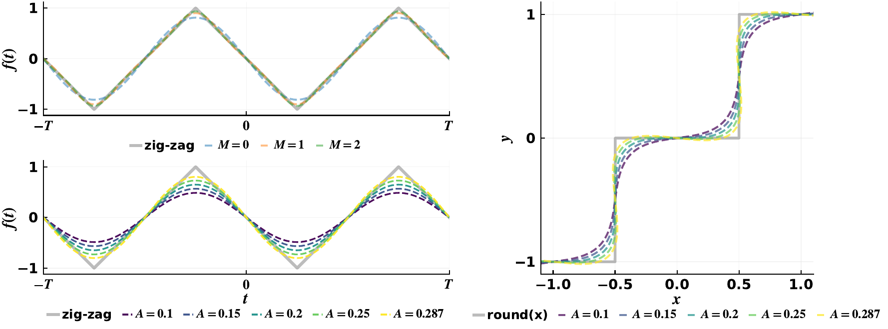
round (right). The amplitude A sets how sharply the surrogate tracks the true step.
Figure from the paper's LaTeX source — Chen et al. (2026), arXiv:2601.19320
Two things about are worth stating plainly because they are what the method rests on, and both are checkable. First, STE is the case: set the amplitude to zero and , exactly the straight-through gradient. So this is not an alternative to STE so much as a one-parameter family that contains it, and dials how much rounding structure to inject. Second, the surrogate is not flat. Because reduces to twice an integer plus the rounding residual , depends only on , and it is largest () at the half-integer boundaries where rounding actually jumps and smallest at the cell centres where rounding is flat. I checked this: at the default amplitude the centre value is and the boundary value is . That is the opposite of STE’s uniform 1, and closer to the truth that rounding’s action is concentrated at its jumps.
The amplitude is the whole ballgame
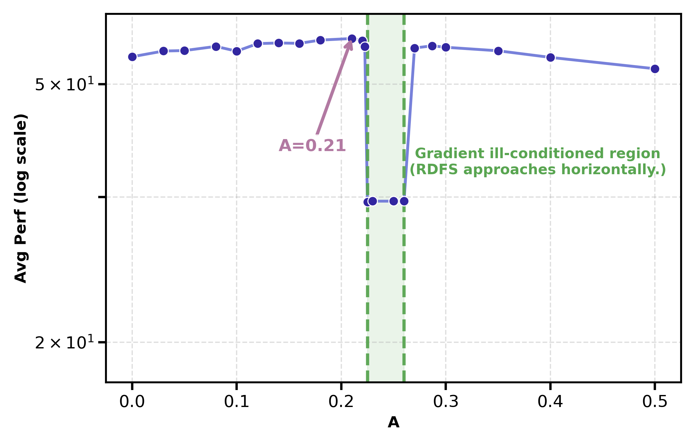
controls sharpness, and it has a narrow safe range that took me a moment to see. Write . The surrogate at a cell centre is . For it is strictly positive, so the gradient keeps its sign everywhere and training is well-behaved. At , i.e. , the centre value hits zero: the surrogate goes tangent to the staircase’s flat plateaus and the gradient there vanishes. Past that, , the numerator goes negative near the centres and the surrogate flips the gradient’s sign, which is as bad as it sounds. The catch the paper is honest about: the mathematically natural Fourier amplitude, , gives , which is already in the sign-flip regime. I verified that at that amplitude the centre gradient is . So the untuned surrogate is broken, and the method’s practicality depends entirely on damping down into the well-conditioned window. They use for everything, just below the boundary.
Why it is supposed to be stable
The paper gives two theorems. The first is an statement: among trigonometric polynomials of degree at most , the th partial Fourier sum is the unique best approximation to the rotated rounding function, and for it is strictly better than any constant unless the target is constant. STE is the degree-0 (constant) case, so StableQAT’s surrogate is provably a closer fit to the rounding operator than STE. The second theorem is the stability argument, and it is the one that distinguishes StableQAT from soft quantizers: as each surrogate is sharpened toward hard rounding, DSQ’s gradient variance diverges to infinity, while StableQAT’s stays bounded. I verified the StableQAT side both by hand and by Monte Carlo: as , the surrogate over a uniform residual becomes , whose mean is exactly and whose variance is exactly , finite. A bounded-variance gradient is the concrete meaning of “stable” here: it cannot explode as the surrogate sharpens, whereas a sigmoid/tanh soft rounder can.
Cost: a cosine, not an exp
The surrogate is a single cosine and a division, with no auxiliary state and no annealing schedule, so its backward pass costs about what STE’s does. That is the practical argument against soft quantizers: DSQ and its relatives approximate rounding with a tanh or sigmoid, which evaluates an exp, and exp is expensive and register-hungry on GPUs relative to a bounded trigonometric call. The paper’s microbenchmark on Llama-3-1B bears it out: StableQAT matches STE in both backward time and memory, while DSQ is several times heavier on both.
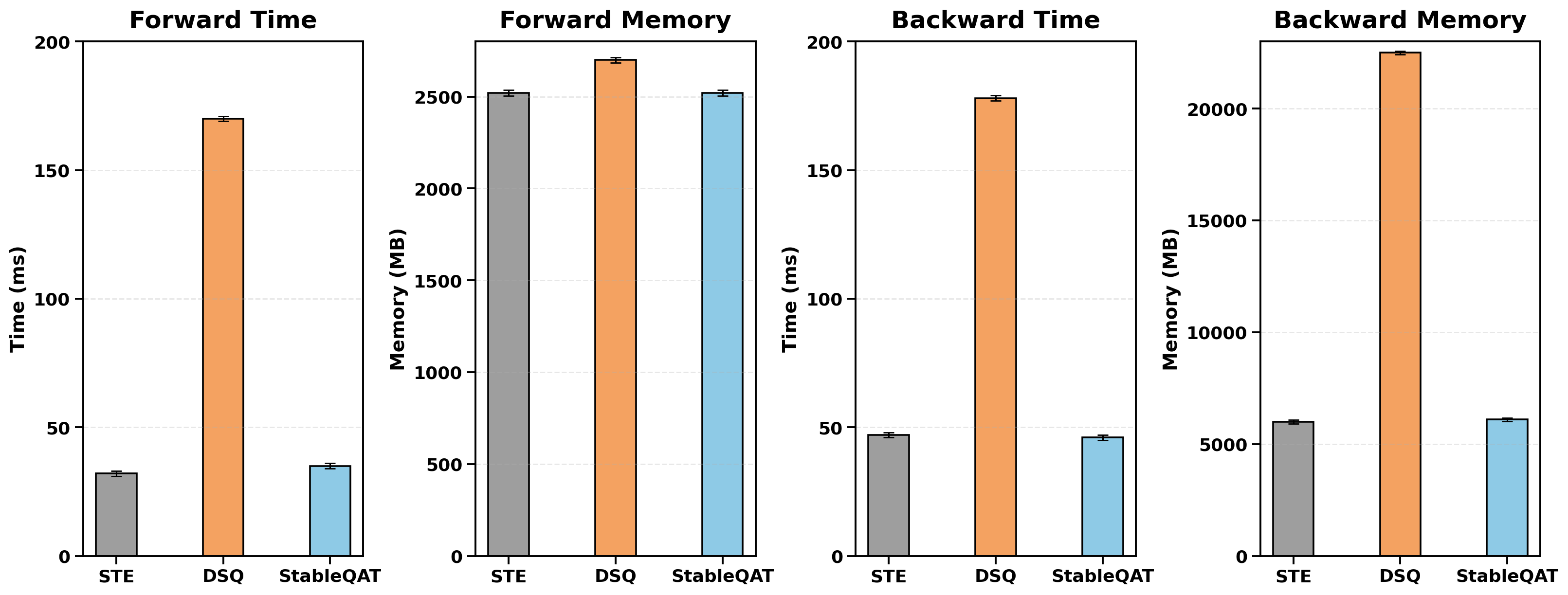
exp-based surrogate (orange) costs several times more in time and in backward memory (forward memory, which the rounding surrogate does not dominate, is close for all three).
Figure from the paper's LaTeX source — Chen et al. (2026), arXiv:2601.19320
Paper vs. code
Repo: microsoft/StableQAT at commit 4760535, official. The quantizer is models/utils_quant.py (400 lines); the surrogate is a handful of lines inside two autograd functions.
What I could match directly:
| Paper | Code |
|---|---|
| First-order RDFS surrogate | utils_quant.py:197–201 (regular) and :43–49 (the @torch.compile “efficient” kernel); I verified both compute the identical |
| STE as the special case | sine_soft_q['enable'] = False takes the else branch grad_input = indicate_middle * grad_output, utils_quant.py:204 |
| Default amplitude , first order | train_configs/.../*_amp_0.21_*fft1*.yaml: amplitude: [0.21] |
| LSQ round-and-clamp forward | utils_quant.py:136, 141; verified 2-bit grid |
| Learned per-channel step size | weight_clip_val, shape (rows, 1), utils_quant.py:364 |
What the code does that the paper doesn’t say:
- The forward quantizer is plain LSQ, not ParetoQ’s zero-free SEQ grid, even though the same file ships
StretchedElasticQuant(SEQ, lifted from ParetoQ) unused in the StableQAT path. So StableQAT’s own contribution is entirely in the backward pass; the grid is the ordinary asymmetric integer set with a zero level. This matters for reading the tables: the ParetoQ and DSQ baselines are run from their own repos (the paper says so), so those comparisons vary the forward grid too, and the cleanest apples-to-apples test of the surrogate is StableQAT against its own limit, which the tables fold into the “STE is a special case” framing rather than isolating. - The paper writes the higher-order surrogate with explicit damping factors, but the code’s
amplitudeis just a coefficient vector the caller supplies; for the first order it is[0.21], and any higher-order damping would have to be baked into that vector by hand. - The surrogate coefficients are pushed to the GPU at construction (
utils_quant.py:368, a bare.cuda()), so the quantizer is CUDA-only as written. - The released configs and README cover Llama-3.2-1B (and 3B configs exist), while the paper also reports Vision Transformers in its appendix; there is no ViT code in this release.
Claims & evidence
Zero-shot average is over eight tasks (ARC-e/c, BoolQ, HellaSwag, OpenBookQA, PIQA, SciQ, WinoGrande) via lm-eval-harness.
| Claim | Evidence in paper | Verdict |
|---|---|---|
| STE is a strict special case () of the surrogate | Method section; L2 theorem (degree-0 case) | verified — exact, at (my check) |
| Gradient variance stays bounded as the surrogate sharpens, unlike DSQ | Their variance theorem | verified for the StableQAT limit (, ) analytically and by MC; the DSQ-divergence half I read but did not re-derive |
| Beats ParetoQ and DSQ at 2–4 bit on Llama-3.2-1B, up to +6.88 | Table 1, eight-task average | verified as reported; largest gap at 3-bit / low-token / high-lr, where the baselines nearly collapse |
| Negligible overhead vs STE, ~1.43× faster than DSQ | Table 1 SpeedUp column (end-to-end) plus the efficiency microbenchmark | verified as reported; consistent with cosine-vs-exp |
| 4-bit exceeds the FP16 baseline | Table captions, both sizes | partial — true for 1B (61.24 vs 60.45) but not 3B, where 4-bit is 67.15 vs 68.46 despite the caption and text saying it surpasses FP16 |
| Stable at 2-bit where baselines have high variance / collapse | Error-bar figure | partial — holds on 1B; on 3B at 2-bit StableQAT (63.05) loses to DSQ (63.78), which the paper reports honestly |
Benchmarks
Llama-3.2-1B, eight-task zero-shot average (higher is better), from the paper’s Table 1. The three differ chiefly in the rounding-gradient surrogate: ParetoQ uses STE, DSQ a tanh soft rounder, StableQAT the RDFS. The baselines are run from their own repos, though, so their forward grids are not identical to StableQAT’s LSQ one (the caveat under Paper vs. code), and the comparison is not a pure surrogate swap.
| Bits | Setting | ParetoQ (STE) | DSQ | StableQAT | FP16 |
|---|---|---|---|---|---|
| 4 | 10B tok, lr 1e-5 | 57.24 | 56.49 | 57.87 | 60.45 |
| 4 | 20B tok, lr 1e-4 | 60.96 | 61.07 | 61.24 | 60.45 |
| 3 | 10B tok, lr 1e-5 | 38.92 | 38.30 | 45.18 | 60.45 |
| 3 | 20B tok, lr 2e-4 | 59.57 | 57.42 | 60.12 | 60.45 |
| 2 | 30B tok, lr 1e-4 | 57.29 | 56.39 | 58.08 | 60.45 |
The row that carries the argument is 3-bit at the aggressive low-token, high-learning-rate setting: ParetoQ and DSQ land at 38.9 and 38.3, barely above the 33.8 of the un-trained 3-bit model, while StableQAT reaches 45.2. That is the instability the method targets: at a hard bit-width with a punishing schedule, STE and soft rounding stall and the Fourier surrogate keeps making progress. At the gentler schedules the margins shrink to a point or less, which is the honest shape of the result.
Limitations & open questions
The evidence is small-model and weights-only. Llama-3.2-1B and 3B are the LLM experiments; there is no 7B/8B point where the ParetoQ and QuIP families live, and activations stay full precision, so this says nothing about the W4A4 regime the activation-outlier methods fight over.
The surrogate rides on a standard LSQ grid, and the obvious experiment is missing: RDFS on top of ParetoQ’s SEQ grid, which is the actual 2-bit state of the art. The two ideas are orthogonal (one is a grid, one is a gradient), the code already contains both quantizers, and nobody has combined them.
The amplitude window is narrow and the default is a fixed constant. The admissible range is , the untuned Fourier value sits outside it, and was chosen by the sweep in the figure above. The paper flags a dynamic or scheduled as future work; as shipped, one global constant carries every model and bit-width.
At 2-bit on the 3B model StableQAT loses to DSQ, and its 3B 4-bit number does not actually beat FP16, both against the paper’s own framing. The method’s strongest, cleanest wins are at 3-bit; the 2-bit story is “stable and competitive,” not “best.”
And it is a preprint in ICML-submission form, not yet peer-reviewed. The theory I checked holds, but the headline accuracy numbers are single-source and, per this site’s usual caveat, transcribed rather than reproduced.
Reproduction notes
Marked partial. On 2026-07-18 I read models/utils_quant.py, models/utils_quant_dsq.py, train.py, and the training configs end to end at commit 4760535 and matched them to the paper; that is the Paper-vs-code section. I reimplemented the first-order surrogate in NumPy and verified: STE is the member (, exact); the conditioning boundary at where the surrogate touches zero, with the untuned Fourier amplitude overshooting into a sign flip; the variance theorem’s StableQAT limit (, ) by hand and by Monte Carlo; and that the forward grid is standard LSQ, independent of . The script is verification/stableqat/checks.py, all PASS. Figures are converted from the arXiv LaTeX source.
What I did not do: run any QAT training (no GPU here) or re-evaluate the released checkpoints, so every accuracy, perplexity, and speed number is the paper’s as reported. The DSQ-variance-divergence half of the stability theorem I read and found plausible but did not re-derive or simulate.