Learned step-size quantization, LSQ and SEQ

Core insights. A uniform quantizer is completely described by one number per layer: the step size $s$ , the width of a quantization bin. Everything else (which integer each weight maps to, the dequantized value) follows. Before LSQ, that step size was set from statistics of the weights or by minimizing quantization error. LSQ’s idea is to treat $s$ as an ordinary learnable parameter and descend the task loss on it, alongside the weights. Two things made that work: a step-size gradient, derived through the straight-through estimator, that grows as a value nears a rounding boundary (because that value is about to jump bins); and a scale factor $1/\sqrt{N\,Q_P}$ on that gradient, so a step size shared by $N$ weights gets updates proportioned like the weights’ own. SEQ, from ParetoQ, is the same learned step size with a differently-shaped grid for the extreme low-bit regime. The learned step size is the quiet substrate under most of this site’s QAT notes, and this is where it comes from.

The step size is the parameter

Take a uniform symmetric quantizer. Given a weight $v$ and a step size $s$ , LSQ (the paper says, Eq. 1–2) computes an integer code and a dequantized value:

\bar v = \big\lfloor \operatorname{clip}(v/s,\ -Q_N,\ Q_P)\big\rceil , \qquad \hat v = \bar v \cdot s .

$\lfloor\cdot\rceil$ is round-to-nearest; for $b$ -bit signed weights $Q_N = 2^{b-1}$ and $Q_P = 2^{b-1}-1$ (so 2-bit weights land on $\{-2,-1,0,1\}\cdot s$ , 4-bit on $\{-8,\dots,7\}\cdot s$ ; I verified both). At inference the integer codes $\bar v$ feed low-precision matrix multiplies and the output is rescaled by $s$ , so $s$ is genuinely the only continuous knob.

The question LSQ answers is how to set $s$ . Earlier methods fit it to the data (match the range, or minimize $\lVert \hat v - v\rVert$ ). LSQ’s argument is that minimizing quantization error is the wrong target: a grid that reproduces the weights most faithfully need not be the grid that preserves the task. So it learns $s$ by gradient descent on the training loss, like any other parameter. The obstacle is the same one every QAT method hits, the round in $\bar v$ has zero gradient almost everywhere, and the interesting part is how LSQ gets a useful gradient to $s$ out of it.

The gradient, and why its shape matters

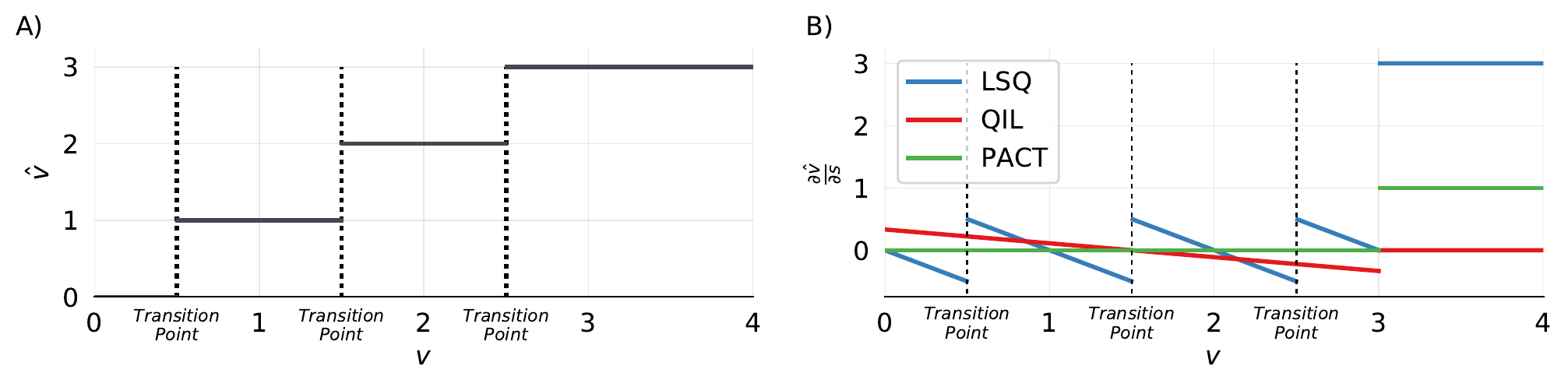
Differentiate $\hat v = \lfloor v/s \rceil \cdot s$ with respect to $s$ , using the straight-through estimator for the round (treat $\partial\lfloor z\rceil/\partial z = 1$ while leaving the round in the forward value). In the interior the product rule gives $\hat v' = (-v/s^2)\,s + \lfloor v/s\rceil = \lfloor v/s\rceil - v/s$ ; in the clipped regions $\bar v$ is a constant so $\hat v' = \mp Q_N,\ Q_P$ . That is LSQ’s Eq. 3:

\frac{\partial \hat v}{\partial s} = \begin{cases} \lfloor v/s\rceil - v/s & -Q_N < v/s < Q_P \\ -Q_N & v/s \le -Q_N \\ Q_P & v/s \ge Q_P . \end{cases}

The interior term is the negative rounding residual, and its magnitude is the distance from $v/s$ to the nearest bin centre: near zero at a centre, near $\tfrac12$ at a transition. That is the property the paper cares about and the earlier methods lacked. A value sitting close to a bin boundary is the one most likely to flip codes when $s$ moves a little, so it should pull hardest on $s$ , and LSQ’s gradient does exactly that while QIL’s is insensitive to boundary distance and PACT’s is zero below the clip point. I verified the three-region formula matches the reference code line for line, and that the interior magnitude stays in $[0,\tfrac12]$ , peaking at the transitions.

Two panels for a quantizer with s=1, Qn=0, Qp=3. Left: the quantizer output v-hat as a staircase in v, flat between transition points. Right: the gradient of v-hat with respect to the step size s. The LSQ curve is a descending sawtooth: it slopes down to about -0.5 just before each transition, then jumps back up to about +0.5 just after it, and jumps to 3 above the top clip; QIL is a single downward-sloping line; PACT is flat at zero below the clip. — **What LSQ learns from.** Left, the quantizer staircase (shown for an unsigned 4-level activation quantizer). Right, the step-size gradient: LSQ's (blue) grows as a value approaches a rounding transition and jumps to $Q_P$ past the clip, whereas QIL (red) ignores transition distance and PACT (green) is flat below the clip. Figure from the paper's LaTeX source — Esser et al. (2020), arXiv:1902.08153

Balancing the step-size update

There is a second, less glamorous contribution that the paper is right to insist on. A single step size is shared by all $N$ weights in a layer, and its gradient sums a residual-sized term over all of them, so its raw magnitude grows like $\sqrt{N}$ (the sum of $N$ roughly independent, zero-mean terms). Meanwhile each weight’s gradient is a single term. Left alone, the step size takes updates two to three orders of magnitude larger than the weights relative to its own size, which the paper measured and which wrecks convergence. LSQ multiplies the step-size gradient by

g = \frac{1}{\sqrt{N\,Q_P}} ,

so that the ratio of update magnitude to parameter magnitude is about the same for $s$ as for the weights. The $1/\sqrt N$ cancels the summing-over- $N$ growth; the $1/\sqrt{Q_P}$ offsets the fact that a finer grid (larger $Q_P$ ) uses a smaller step, so its gradient would otherwise scale differently with precision. I verified the $\sqrt N$ part directly: the summed step-size gradient’s magnitude tracks $\sqrt N$ across four orders of magnitude, so dividing by $\sqrt N$ flattens it. This gradient-scaling trick is not incidental; it reappears verbatim as the $1/\sqrt{n\,Q_p}$ factor in ParetoQ’s and StableQAT’s code.

The remaining details: $s$ is initialised to $2\langle|v|\rangle/\sqrt{Q_P}$ from the initial weights, the first and last layers are left at 8 bits, and training fine-tunes from a full-precision model. On ImageNet this was the state of the art of its day (paper says): ResNet-18 at 2/3/4 bits scored 67.6 / 70.2 / 71.1 against a 70.5 full-precision baseline, so 4-bit exceeds full precision and 3-bit lands within a few tenths, with the paper reporting 3-bit matching full precision once knowledge distillation is added.

SEQ: the same knob, a better low-bit grid

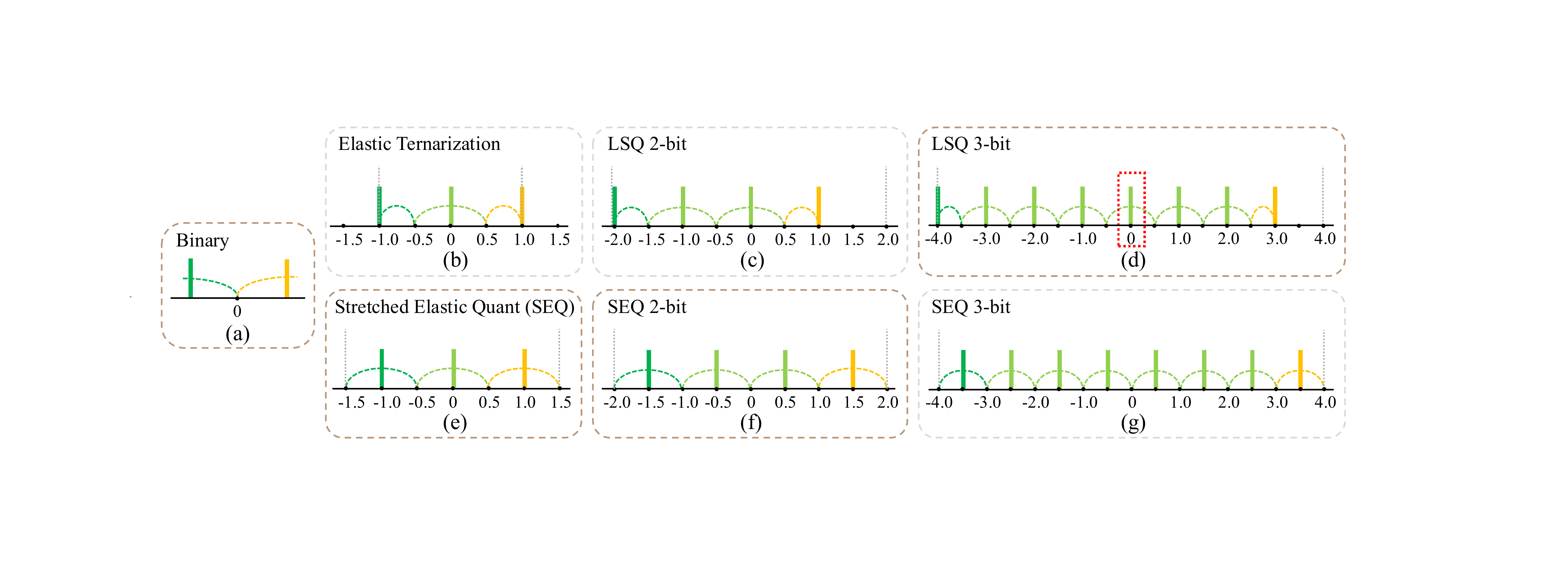
LSQ’s grid is the plain integer set, and it carries two features that are invisible at 4 bits and expensive at 2. It contains zero, which costs a level, and it is asymmetric, one more negative level than positive. At sixteen levels nobody notices; at four levels, $\{-2,-1,0,1\}$ spends its budget on a single positive value and a zero. ParetoQ introduced Stretched Elastic Quant (SEQ) to fix exactly this, and it is not a separate paper or a new training method, it is LSQ’s learned step size with the grid reshaped. SEQ keeps the learnable $\alpha$ (its name for $s$ ) and the three-region gradient, but replaces the integer round with

\hat w = \alpha\cdot\frac{\big\lfloor \operatorname{clip}(w/\alpha,\ \pm 0.99)\cdot k - \tfrac12\big\rceil + \tfrac12}{k}, \qquad k = 2^{b-1},

whose half-integer shift lands the levels on symmetric, zero-free bin centres. I verified the grids from the code: 2-bit SEQ gives $\{-0.75,-0.25,+0.25,+0.75\}\,\alpha$ , four balanced values with no zero, and ternary SEQ gives $\{-\tfrac23,0,+\tfrac23\}\,\alpha$ , keeping zero only where an odd level count makes it free. ParetoQ’s ablations pick SEQ for ternary and 2-bit and plain LSQ for 3 and 4, which is the crossover made concrete: the zero-free symmetric grid wins exactly when levels are scarce.

Quantization grid diagrams. Top row shows standard grids including a 2-bit LSQ grid with levels -2,-1,0,1 and a red box marking its imbalanced extra negative level. Bottom row shows SEQ grids at ternary, 2-bit and 3-bit whose levels are symmetric about zero and evenly divide the clipped range. — **LSQ vs SEQ where it matters.** The 2-bit LSQ grid (top, with the imbalanced level boxed) against SEQ's symmetric zero-free set (bottom). Same learned step size, different placement; the difference is worth several points at four levels and nothing at sixteen. Figure from ParetoQ's LaTeX source — Liu et al. (2025), arXiv:2502.02631

Where this shows up

LSQ is a 2020 CNN paper, but its learned step size is the substrate under most of the low-bit LLM work on this site. ParetoQ is LSQ for 3–4 bit and SEQ for 1–2 bit, trained end to end. StableQAT keeps LSQ’s forward and its step-size gradient unchanged, and swaps only the straight-through estimator on the weight gradient (the round’s $\partial x_q/\partial x$ ) for a Fourier surrogate. EfficientQAT learns an affine version (a step size and a zero point) block by block. Even GPTQ, which learns nothing, fits a per-row step size before quantizing. Once you have read the LSQ gradient and its $1/\sqrt{N Q_P}$ scale, that recurring grad_scale = 1/sqrt(numel * Qp) line in every one of these repos stops looking like a magic constant and starts looking like a citation.

What I verified

The checks are one seeded NumPy script, verification/learned-step-size/checks.py, all PASS: the LSQ integer grids (signed 2- and 4-bit, unsigned 2-bit); that the paper’s Eq. 3 step-size gradient equals the reference code’s formula exactly, with the interior magnitude bounded by $\tfrac12$ and peaking at the transitions; that the unscaled step-size gradient grows as $\sqrt N$ , which is what the $1/\sqrt N$ in the gradient scale cancels; and the SEQ 2-bit and ternary grids, with the structural contrast that LSQ’s 2-bit grid has a zero and is asymmetric while SEQ’s is zero-free and symmetric. The LSQ math is from the paper and its LaTeX; the code references are the LsqBinaryTernaryExtension and StretchedElasticQuant implementations in the ParetoQ (7b36b8d) and StableQAT (4760535) repos, which cite LSQ directly. LSQ has no official code release, so the “code does” side is those faithful reimplementations, not the authors’ own. I did not retrain any model; the ImageNet accuracies are the paper’s as reported.